The old adage says to “Sell in May and go away”. That’s simple enough, but it’s less clear when it’s the appropriate time to buy back in. Some traders suggest going long again after Labor Day, which is the first Monday in September. Others completely avoid historically treacherous October and stay away until the beginning of November, a full 6 months!

This old trading adage is based upon the observation that historical returns on the Dow Jones Industrial Average (INDU) for the six months from the beginning of May through to the end of October, underperform compared to the six months from November to April. As well as the fact that there is typically less trading activity during the summer due to vacationing traders.

I decided to perform a bit of analysis in order to find out if there is anything to this claim. Rather than using data from the DJIA, I chose to use data from the S&P 500 index (SPX), and compared simple returns for the six month period from May through October, to the six month period from November through April, for the past 20 years.

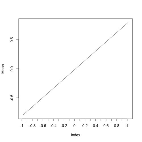
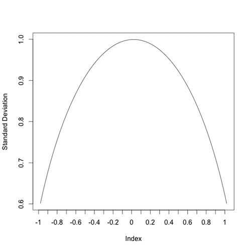
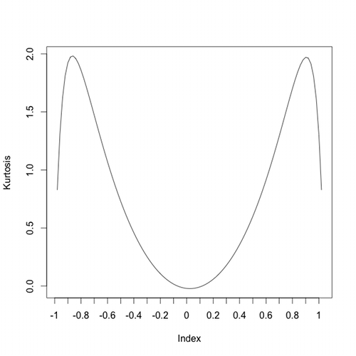
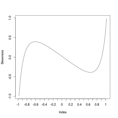
The results from the past 20 years show that there is a somewhat significant difference in average simple returns. For the May through October period, not only is the mean lower, but the standard deviation (i.e. volatility) is higher, the negative skewness is more pronounced, and the excess kurtosis (i.e. long tails) is more severe. All of this historical data appears to back up the conclusion that while the average return for the summer is marginally positive, there is a significant amount of downside risk associated with that return.

From a risk/reward perspective, investors might be better off avoiding the May through October time period. The downside is that investors choosing to follow this strategy will potentially incur higher capital gains taxes due to additional trading. They will also need to commit to this strategy over a long period of time in order to potentially benefit because these are averages over the past 20 years. For any given six month period, simple returns are highly variable and may not conform to the average. Just last year, investors out of the market from May through October missed out on a much higher than expected return of 9.95%.

My son wondered why we don’t have a more rational, decimal system for time. To explore the idea, we made a simple javascript clock implementing decimal time.

We chose a 20 hour day, rather than 10, because it makes the duration of an hour more similar to our current system, and therefore a bit more intuitive as a unit of time.

Time subdivisions

• 20 hours per day; each hour equals 72 standard minutes.
• 100 minutes per hour; each minute equals 43.2 standard seconds.
• 100 seconds per minute; each second equals 0.432 standard seconds.
  Midnight, 6am, noon, and 6pm align with the hours 0, 5, 10, and 15.

The half-normal distribution is a special case of the folded normal distribution, where if X is a standard normal distribution, the absolute value of X is the half-normal distribution.

The mean of the half-normal distribution:
halfNormalMean <- sqrt(2 / pi)

The standard deviation of the half-normal distribution:
halfNormalSD <- sqrt(1 - (2 / pi))

The skewness of the half-normal distribution:
halfNormalSkewness <- sqrt(2) * (4 - pi) / (pi - 2) ^ (3 / 2)

The kurtosis of the half-normal distribution:
halfNormalKurtosis <- 8 * (pi - 3) / (pi - 2) ^ 2

There is an exact linear relationship between the mean of a standard normal variable and the mean of a folded variable as an increasing percentage of values from the sample are folded (i.e. their absolute value is taken). There is a corresponding parabola-like relationship between the standard deviation of a standard normal variable and a half-normal variable.

Here is a quick example, allowing the incremental folding of values. The plots show the change in the mean, standard deviation, skewness, and excess kurtosis as the values are incrementally folded over the range from -abs(x) --> x --> abs(x). Notice the linear change of the mean and the near parabolic change of the standard deviation.

# to provide the kurtosis and skewness functions
library(PerformanceAnalytics)

upDown <- c(0:50, 49:0)
downUp <- c(50:0, 1:50)    # 50 - upDown
s <- c(rep(-1, 50), rep(1, 51))

x <- rnorm(100000)

m101 <- matrix(nrow = 101, ncol = 4)

for (i in 1:101) {
  tmp <- c(rep(x, upDown[i]), rep(s[i] * abs(x), downUp[i]))

  m101[i, 1] <- mean(tmp)
  m101[i, 2] <- sd(tmp)
  m101[i, 3] <- skewness(tmp)
  m101[i, 4] <- kurtosis(tmp)
}

colnames(m101) <- c("Mean", "SD", "Skewness", "Kurtosis")