Half-normal Distribution

The half-normal distribution is a special case of the folded normal distribution, where if X is a standard normal distribution, the absolute value of X is the half-normal distribution.

The mean of the half-normal distribution:
halfNormalMean <- sqrt(2 / pi)

The standard deviation of the half-normal distribution:
halfNormalSD <- sqrt(1 - (2 / pi))

The skewness of the half-normal distribution:
halfNormalSkewness <- sqrt(2) * (4 - pi) / (pi - 2) ^ (3 / 2)

The kurtosis of the half-normal distribution:
halfNormalKurtosis <- 8 * (pi - 3) / (pi - 2) ^ 2

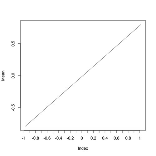
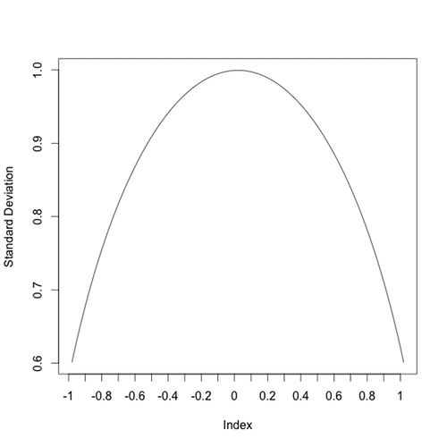
There is an exact linear relationship between the mean of a standard normal variable and the mean of a folded variable as an increasing percentage of values from the sample are folded (i.e. their absolute value is taken). There is a corresponding parabola-like relationship between the standard deviation of a standard normal variable and a half-normal variable.

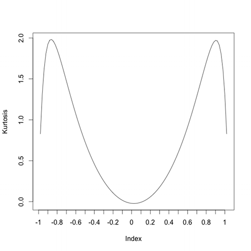
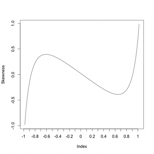
Here is a quick example, allowing the incremental folding of values. The plots show the change in the mean, standard deviation, skewness, and excess kurtosis as the values are incrementally folded over the range from -abs(x) --> x --> abs(x). Notice the linear change of the mean and the near parabolic change of the standard deviation.

# to provide the kurtosis and skewness functions
library(PerformanceAnalytics)

upDown <- c(0:50, 49:0)
downUp <- c(50:0, 1:50)    # 50 - upDown
s <- c(rep(-1, 50), rep(1, 51))

x <- rnorm(100000)

m101 <- matrix(nrow = 101, ncol = 4)

for (i in 1:101) {
  tmp <- c(rep(x, upDown[i]), rep(s[i] * abs(x), downUp[i]))

  m101[i, 1] <- mean(tmp)
  m101[i, 2] <- sd(tmp)
  m101[i, 3] <- skewness(tmp)
  m101[i, 4] <- kurtosis(tmp)
}

colnames(m101) <- c("Mean", "SD", "Skewness", "Kurtosis")